How Does the NFL Use Facebook? An Excuse to Connect to the Facebook API Using R

A couple of weeks ago, I stumbled on a neat blog - "Think to Start". On think to Start he has a number of tutorials with R. The tutorials have clear business applications, so  I decided to try a few out. 

When playing around with the Facebook Open Graph API, I realized that you could pull out data for posts from any public Facebook page. With each post, you also get dimensions like time posted, day of the week and the number of likes, comments, and shares. 

With this API I was able to capture this data for 1,338 updates from the official NFL Facebook page (Facebook.com/NFL), from 10/24/12 to 12/04/14.

With a little data clean up, we can do some very cursory, yet pretty interesting analysis with both R and excel. 

The first thing I wanted to do, after cleaning up the data, was to visualize it to see if there was anything unexpected or surprising. 

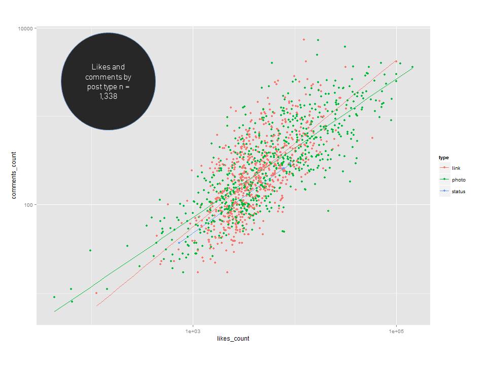
Once we brought in those initial visualizations, I wanted to dig a little deeper. I added some median lines and added a histogram for the number of likes, comments and shares by post type.

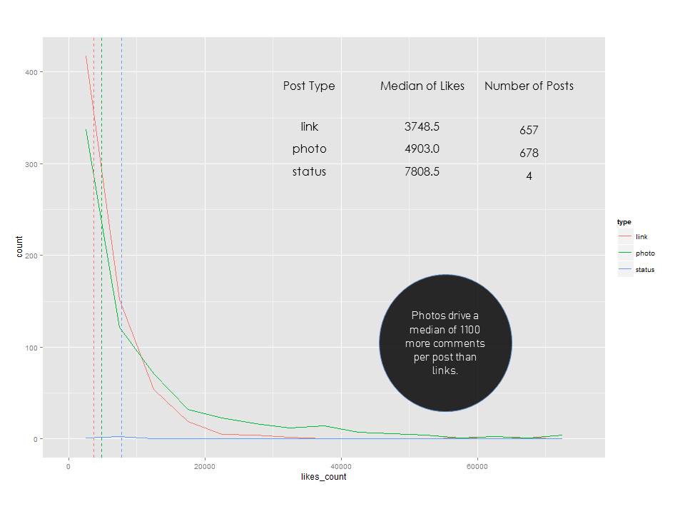
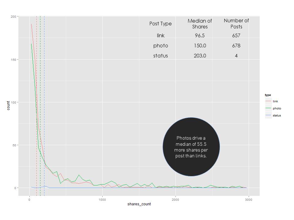
After seeing these histograms, I really wanted to understand the distribution a little better by overlapping post types.

I think it's pretty clear now that photos outperformed the "status" update type in terms of driving fan engagement for the NFL. If we know that post type has some sort of an impact on the amount of engagement, what about the day of the week? 

Hmmm - It seems that engagement follows a pretty specific pattern...

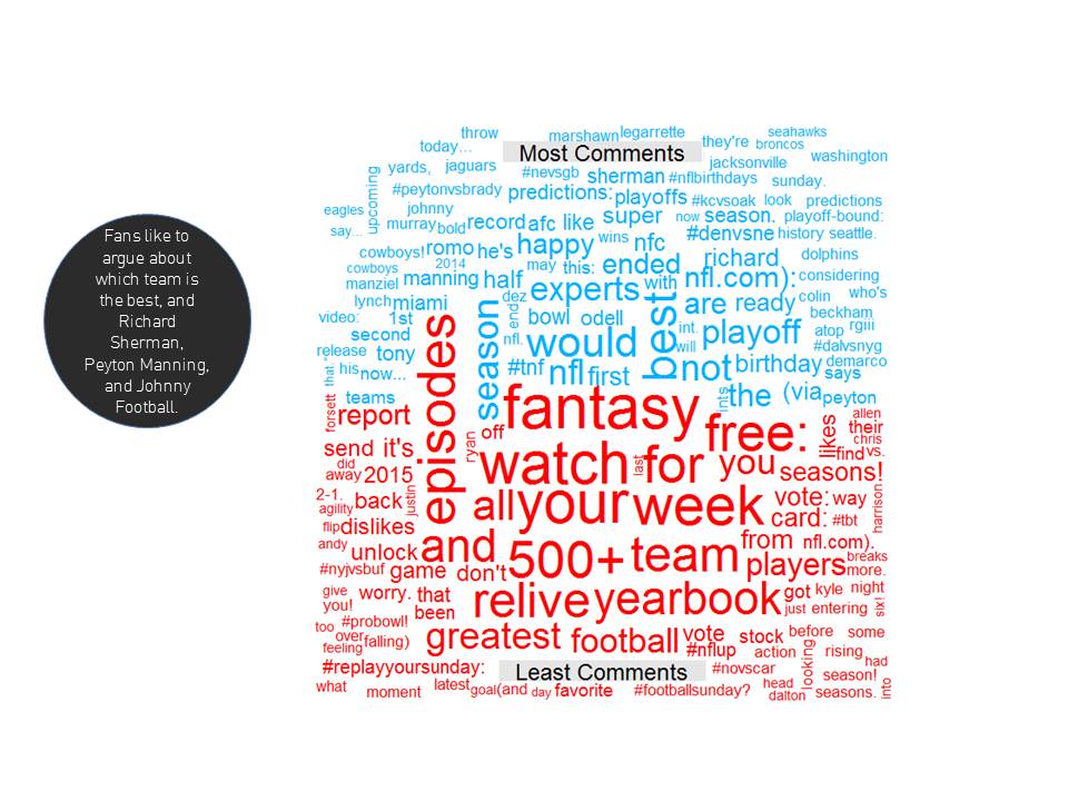
Now that we've figured out that the NFL can literally not post ENOUGH, it got me thinking about the content of the updates themselves. Was there any way to do some text mining to figure out the frequency of certain words and how they drive specific types of engagements? Using R again, I was able to create a word cloud which omits common words where the words are sized based on frequency. There isn't that much to be learned here yet - The NFL talks a lot about specific players, teams, fantasy football and itself. 

What happens when we compare the frequency of words in the 100 posts that are most liked versus 100 least liked? This is starting to get more interesting. People sure do love to wish their favorite player happy birthday with a "like." 

What about the 100 most commented on posts versus the least commented on posts?  You can see that there are a couple of players here that drive a lot of "discussion." Specifically Richard Sherman, Peyton Manning, and Johnny Manziel. Again - no one is interested in re-watching games or engaging with NFL promotions. 

What about word frequency in content that is the most or least shared? That amazing Odell Beckham catch dominates, as well as specific marquee games. 

Pretty interesting, to summarize:

1) The NFL posts a lot on Facebook , evenly distributed between links and photos.

2) Photos drive more engagement than links.

3) The favorite day for the NFL to post is on Monday, and that is also the day where the is the highest amount of fan engagement per post. 

4) The amount of engagement per post fits with the average number of posts per day (R squared of .42), suggesting that the NFL could be posting even more.

5) If you want to start a flame war with NFL fans - bring up Peyton Manning, Johnny Manziel or Richard Sherman. I can't guarantee that the comments will be worth reading however :)

I've included the code below for bringing the posts in, the visualizations and the wordcloud comparison. 

Use RFacebook to bring in posts

Connect to Facebook require(Rfacebook) token <- “YOURTOKENHEREFROMOPENGRAPHAPI" #Pull in Posts number_posts <- 3200 #Define Your PageName page_name <- “NFL" #Get Posts page <- getPage(page_name, token, n = number_posts) #Export and Clean Data – Remove posts with “NA” in message field in Excel write.csv(page, file = “NFLOverview.csv") #Visluaziation 1 - Scatter Plot NFLOVerview2 <- NFLOverview[-which(log(NFLOverview2 $likes_count) <= 0), ] NFLOVerview2 <- NFLOverview[-which(log(NFLOverview2 $comments_count) <= 0),] NFLOVerview2 <- NFLOverview[-which(log(NFLOverview2 $shares_count) <= 0), ] ggplot(NFLOVerview2, aes(x=shares_count, y=comments_count, color=type)) + geom_smooth(aes(group=type), se=F, method=lm) + geom_point() + scale_y_log10() + scale_x_log10() #Define Meansand Medians - Define Means and Medians For Likes, Comments, Shares LikesMean <- ddply(NFLOverview2, "type", summarise, likes_count.mean=mean(likes_count)) CommentsMean <- ddply(NFLOverview2, "type", summarise, comments_count.mean=mean(comments_count)) SharesMean <- ddply(NFLOverview2, "type", summarise, shares_count.mean=mean(shares_count)) LikesMedian <- ddply(NFLOverview2, "type", summarise, likes_count.median=median(likes_count)) CommentsMedian <- ddply(NFLOverview2, "type", summarise, comments_count.median=median(comments_count)) SharesMedian <- ddply(NFLOverview2, "type", summarise, shares_count.median=median(shares_count)) #Visluaziation 2 - geometric frequency plot with added lines for means ggplot(NFLOverview2, aes(likes_count, color = type)) + geom_freqpoly(binwidth = 5000)+ xlim(0, 75000) + geom_vline(data=LikesMedian, aes(xintercept=likes_count.median, colour=type),linetype="dashed", size=.25) ggplot(NFLOverview2, aes(comments_count, color = type)) + geom_freqpoly(binwidth = 500)+ xlim(0, 5000) + geom_vline(data=CommentsMedian, aes(xintercept=comments_count.median, colour=type),linetype="dashed", size=.25) ggplot(NFLOverview2, aes(shares_count, color = type)) + geom_freqpoly(binwidth = 50)+ xlim(0, 3000) + geom_vline(data=SharesMedian, aes(xintercept=shares_count.median, colour=type),linetype="dashed", size=.25)

Create Frequency Word Cloud

# Read File file_loc <- "FILEDIRECTORY" # change TRUE to FALSE if you have no column headings in the CSV x <- read.csv(file_loc, header = TRUE) #Turn File into Corpus require(tm) corp <- Corpus(DataframeSource(x)) # Clean Data corp <- tm_map(corp, removePunctuation) corp <- tm_map(corp, removeNumbers) corp <- tm_map(corp, removeWords, stopwords("english")) corp <- tm_map(corp, tolower) corp <- tm_map(corp, removeWords,"football") require(SnowballC) corp <- tm_map(corp, stemDocument) # Turn data into Term Document Matrix tdm <-termdocumentmatrix mydata="x" o:p="corp" inspect(corp [1:5]) corp <- tm_map(corp, stripWhitespace) dtm <- TermDocumentMatrix(corp) m <- as.matrix(tdm) v <- sort(rowSums(m),decreasing=TRUE) d <- data.frame(word = names(v),freq=v) # Wordcloud wordcloud(words = d$word, freq = d$freq, min.freq = 2, max.words = Inf,random.order = FALSE, colors=brewer.pal(8, "Dark2"))

Create Comparison Word Cloud From Two CSVs

#File 1 – CSV with 100 posts with least likes, just text file_loc <- "FileDirectoryForFirstFile" # change TRUE to FALSE if you have no column headings in the CSV y <- read.csv(file_loc, header = TRUE) require(tm) LeastLikes <- Corpus(DataframeSource(y)) LeastLikes <- tm_map(corp, removePunctuation) LeastLikes <- tm_map(corp, removeNumbers) LeastLikes <- tm_map(corp, removeWords, stopwords("english")) LeastLikes <- tm_map(corp, removeWords,"football") LeastLikes <- tm_map(corp, tolower) #File 2 – CSV with 100 posts with most likes, just text file_loc <- ""FileDirectoryForSecondFile"" # change TRUE to FALSE if you have no column headings in the CSV x <- read.csv(file_loc, header = TRUE) require(tm) MostLikes <- Corpus(DataframeSource(x)) MostLikes <- tm_map(corp2, removePunctuation) MostLikes <- tm_map(corp2, removeNumbers) MostLikes <- tm_map(corp2, removeWords, stopwords("english")) MostLikes <- tm_map(corp2, removeWords,"football") MostLikes <- tm_map(corp2, tolower) all = c(x,y) c(stopwords("english"), "football", "the", "are",) corpus = Corpus(VectorSource(all)) require(tm) all <- tm_map(corpus, removePunctuation) all <- tm_map(corpus, removeNumbers) all <- tm_map(corpus, tolower) tdm = TermDocumentMatrix(corpus) tdm = as.matrix(tdm) colnames(tdm) = c("Most Likes", "Least Likes") comparison.cloud(tdm, random.order=FALSE, colors = c("#00B2FF", "red", "#FF0099", "#6600CC"), title.size=1.5, max.words=250)aes(xintercept=shares_count.mean, colour=type),linetype="dashed", size=.25)